hokudai_hitachi2020_b

## Table Of Contents [Problem Summary](#gaiyou_en) [Time Schedules and Spatial Structures](#time-space_en) [Constitution of a Nanogrid](#nanogrid_en) [Energy Balance](#yojou_en) [Order Processing](#trans_en) [EV Operation](#ev_en) [Charge/Discharge to the Battery of a Nanogrid](#charge_en) [Scoring](#scoring_en) [Problem B](#problem_en) [Input and Output Format 1](#io-format1_en) [Input and Output Format 2](#io-format2_en) [Input and Output Format 3](#io-format3_en) [Constraints for Input and Output](#constraints_en) [Example of Inputs and Outputs](#example_en) [Sample Code B](#sample_en) Problem Summary --------------- In this problem, you operate multiple electric vehicles (EVs) so that you can transport customers and goods from one place to another place efficiently while protecting distributed nanogrids from overloading the electrical supply to EVs and providing additional power from EVs if there is a power shortage in the nanogrids. Since EVs consume electricity proportional to their distances traveled, they need to charge from nanogrids if necessary. Each nanogrid is equipped with a battery, a photovoltaic (PV) power system and a fuel engine. Power generation, consumption and charge/discharge to EVs occur in each nanogrid and their time-varying imbalance is compensated by charge/discharge from the battery and electrical supply from outside.  The toolkit, which can be downloaded from the bottom of this page, contains a sample of contestant code in which input/output such as reading data from the judge code has already been implemented. Also, regarding the operation of EV, "all stay", "random walk", and "multiple transportation" have been implemented as examples. When implementing a new algorithm, the sample is designed so that you can focus on describing the operation of EV by inheriting the strategy class. (See README.md for details.) You can use the sample when submitting your code. Time Schedules and Spatial Structures ------------------------------------- * **Time Schedules**: The total time length of each test case corresponds physically to one business day. The time variable $t$ is supposed to be integer valued ranging from $0$ to $T_{max}$. For each test case, one of the four different one day weather patterns is randomly assigned and the weather pattern affects the resulting time series of difference between generated and consumed powers (energy balance). In the beginning of each test case, each contestant gets a whole time series of predicted energy balance and, for each time $t$, each contestant gets the charged capacity of the battery for each nanogrid, the set of orders assigned so far, and the following values in the previous step: actual energy balance, excess amount of power discarded, and power supplied from the outside. Based on the information, each contestant is asked to decide how to operate multiple EVs in the next step for each time $t$. * **Spatial Structures**: Let $G = (V, E)$ be a simple and undirected graph with the vertex set $V$ and the edge set $E$, which represents a road network on which EV transportation and EV charge/discharge occur. Nanogrids are located on some of the vertices. An edge represents the road connecting its two endpoints and has a positive integer weight corresponding to the road distance. The graph is generated by the algorithm below. Algorithm to generate the graph $G$ For all test cases, the graph $G = (V, E)$ is generated by the following algorithm. * **Input:**$|V|$, $|E|$, $\mathrm{MaxDegree}=5$ * **Algorithm to generate the vertices:** * Find the maximum non-negative integer $R$ such that $|V| = R^{2} + r$ holds for a non-negative integer $r$. * For each lattice point satisfying $0 \leq x, y < R$ in the $xy$ plane, plot a point $(x, y)$. * Shift each point such as $(x, y) \leftarrow (x + dx, y + dy)$ where $dx$ and $dy$ are random numbers sampled uniformly from the interval $[0, 1]$. * Remaining $r$ points are plotted at $(x', y')$ where $x'$ and $y'$ are random numbers sampled uniformly from the interval $[0, R]$. * Assign a separate ID ranging from $1$ to $|V|$ to each point and identify each point to the vertex having the assigned ID. * **Algorithm to generate the $|V|-1$ edges and their weights to guarantee the connectivity of the resulting graph:** * Generate the complete graph $G_{\text{comp}}$ with the vertex set $V$. For each pair of vertices $u, v \in V$, assign the Euclidean distance between the points corresponding to $u$ and $v$ to the edge weight $W_{u,v}$. * Generate [the minimum spanning tree](https://en.wikipedia.org/wiki/Minimum_spanning_tree) for $G_{\text{comp}}$ and add $|V|-1$ edges in the minimum spanning tree to the graph $G$. For each edge $\left{ u, v \right}$, assign $\lceil 2 \times W_{u, v} \rceil $ to the edge weight $d_{u,v}$. * **Algorithm to generate the remaining $|E|-(|V|-1)$ edges and their weights:** * Remaining $|E|-(|V|-1)$ edges are generated by the following algorithm. * Update $\mathrm{cost}(u,v)$ based on the algorithm below. * Find the pair of vertices $u$ and $v$ minimizing $\mathrm{cost(u,v)}$ among all the pairs of vertices not connected by the edges added to the graph $G$ so far and add the edge $\left{ u, v \right}$ connecting the pair to the graph $G$. * Assign $\lceil 2 \times W_{u, v} \rceil $ to the edge weight $d_{u,v}$. * Here $\mathrm{cost}(u,v)$ is basically determined by the Euclidean distance between the points corresponding to $u$ and $v$ but is biased so that a pair of vertices $u$ and $v$ one of whose degree is small and a pair of vertices lining up vertically and horizontally rather than diagonally are likely to be selected. Due to the bias, the resulting graph is expected to be close to a planer graph. In what follows, we show the algorithm to compute $\mathrm{cost}(u,v)$. * Compute the degree $\mathrm{degree}(u)$ of the vertex $u\in V$. The degree $\mathrm{degree}(u)$ of the vertex $u\in V$ is defined by the number of edges incident to the vertex. * Assign a color to each vertex $u\in V$ as follows: Colors of the first added $R^{2}$ vertices are determined based on their original lattice points $(x,y)$ based on the rule below. Colors of the remaining $r$ vertices are randomly assigned to be $0$ or $1$. * If $x+y$ is even : $\mathrm{color}(u) = 0$ * If $x+y$ is odd : $\mathrm{color}(u) = 1$ * Bias factor $f(u,v)$ is determined by the following rule: * If $\mathrm{color}(u) = \mathrm{color}(v)$ ： $\mathrm{f}(u,v) = 5$ * If $\mathrm{color}(u) \neq \mathrm{color}(v)$ ： $\mathrm{f}(u,v) = 1$ * Bias factor $g(u)$ is determined by the following rule: * If $\mathrm{degree}(u) \lt \mathrm{MaxDegree}$ : $g(u)=1$ * If $\mathrm{degree}(u) \geq \mathrm{MaxDegree}$ : $g(u)=\infty$ * Compute $\mathrm{cost}(u,v)$ as follows： * $\mathrm{cost}(u,v) = W_{u,v}\times \mathrm{degree}(u) \times \mathrm{degree}(v) \times f(u,v) \times g(u) \times g(v)$. * **Algorithm to select vertices where nanogrids are located :** * Uniformly and randomly select $N_{\mathrm{grid}}$ distinct vertices from $V$ and locate a nanogrid on each selected vertex. The set of the vertices on which nanogrids are located is denoted as $V_{\mathrm{grid}}$. 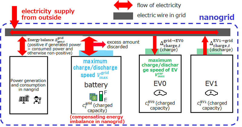Constitution of a Nanogrid -------------------------- Each nanogrid consists of a battery, a photovoltaic (PV) power system, a fuel engine, charging/discharging stations for EVs and power consumers and has the following attributes. * **Vertex ID**: ID of the vertex $u$ on which the nanogrid is located where $u \in V_{\mathrm{grid}}$ ($V_{\mathrm{grid}}$: the set of vertices on which nanogrids are located (See "Algorithm to generate the graph $G$".) ) * **Charged Capacity**: The charged capacity of the battery in the nanogrid. Its initial value is $C_{\mathrm{init}}^{\mathrm{grid}}$ and its maximum value is $C_{\mathrm{max}}^{\mathrm{grid}}$, which are the same for all the nanogrids. For each time $t$, the charged capacity changes by the difference between generated and consumed powers (energy balance) and it also changes by the difference between discharged and charged electricity to EVs (For the detail, see **[Charge/Discharge to the Battery of a Nanogrid](#charge_en)** .). If the resulting charged capacity exceeds $C_{\mathrm{max}}^{\mathrm{grid}}$ at the time $t$, the charged capacity is set to $C_{\mathrm{max}}^{\mathrm{grid}}$ at the time $t+1$ and the excess amount is discarded. Instead, if the resulting capacity is negative at the time $t$, the shortage is supplied from outside and the charged capacity is set to $0$ at the time $t+1$. If the latter is the case, the score is deducted in proportion to the amount of shortage (For the detail, see **[Scoring](#scoring_en)**.) * **Energy Balance**: Difference between generated and consumed powers except for those for charging/discharging EVs for each time $t$. Its predicted value for each time $t$ is provided to contestants in the beginning of each test case. Its actual value is sums of the predicted value and random value caused by stochastic fluctuation of the environment and sudden weather changes like downpour and sudden clear sky (For the detail, see **[Energy Balance](#yojou_en)** below.) * **Maximum charging/discharging speed**: The maximum speed of charging/discharging to the battery $V_{\max}^{\mathrm{grid}}$, which is the same for all the nanogrids. Energy Balance -------------- Difference between generated and consumed powers except for those for charging/discharging EVs for each time $t$. * **Pattern of the time series of the energy balance**: For each test case, one of the four different one day weather patterns, i.e., sunny with/without downpour and rainy with/without sudden clear sky is randomly assigned and is informed to each contestant in the beginning of the test case. For each nanogrid, one of the $N_{\mathrm{pattern}}$ different expected demand patterns is randomly assigned and is informed to each contestant in the beginning of each test case. A whole time series of predicted energy balance is provided to each contestant in the beginning of each test case. The amount of generated powers from the PV power system depends on the weather pattern and thus the sums of the predicted values of energy balance in one business day is largest for the weather pattern, sunny without downpour, and is smallest for the weather pattern, rainy without sudden clear sky. * **The time series of the energy balance**: The time series of the energy balance is sums of predicted one and stochastic fluctuation $\delta$ and the variation due to downpour and sudden clear sky. * The total time interval $0 \leq t < T_{\max}$ is divided into $N_{\mathrm{div}}$ subintervals of equal length and predicted value of the energy balance is constant for each subdivided interval. * For each time $t$, $\delta$ is sampled from the normal distribution with the mean $0$ and the variance $\sigma^{2}_{\mathrm{ele}}$. The variance is informed to each contestant in the beginning of each test case but the value $\delta$ is not informed to each contestant in advance. * Downpour: If the weather pattern is $1$ (sunny with downpour), downpour occurs with a probability $p_{\mathrm{event}}$ for each of $N_{\mathrm{div}}$ subintervals. The probability is constant and independent for each subinterval. If the downpour occurs, the energy balance is subtracted by $\Delta_{\mathrm{event}}$ for $15$ percent of the nanogrids randomly and independently chosen for each subinterval because generated power from a photovoltaic (PV) power system decreases. * Sudden clear sky: If the weather pattern is $3$ (rainy with sudden clear sky), sudden clear sky occurs with the probability $p_{\mathrm{event}}$ for each of the $N_{\mathrm{div}}$ subintervals. If the sudden clear sky occurs, the energy balance is added by $\Delta_{\mathrm{event}}$ for $15$ percent of the nanogrids randomly and independently chosen for each subinterval because generated power from a photovoltaic (PV) power system increases. In case of the weather patterns $1$ and $3$, the timing for downpour or sudden clear sky is not informed to each contestant in advance.  Order Processing ---------------- An order to transport goods from one vertex $u \in V$ to another vertex $v \in V$ is randomly generated based on the algorithm below for each time $t$ and each contestant is asked to process the order by picking it up at the vertex $u$ and delivering it to the vertex $v$ by operating EVs. In what follows, we call $u$ a starting vertex and $v$ a destination vertex. * **Attributes for order**: * Order ID $(1,...)$ * Load time $(0 \leq t \leq T_{\mathrm{last}}(<T_{\max}))$ * Starting vertex $(1,...,|V|)$ * Destination vertex $(1,...,|V|)$ * State ($0$ if none of the EVs picks the order up and $1$ if one of the EVs picked it up but it is not yet delivered.) * **Algorithm to generate orders**: For each time $t$ satisfying $0 \leq t \leq T_{\mathrm{last}}(<T_{\max})$, a new order is randomly generated with the probability $p_{\mathrm{trans}}^{\mathrm{const}}$. Its starting vertex is randomly selected from the vertex set $V$ and its destination vertex is randomly selected from all the vertices except for the starting vertex. * **Penalty for outstanding orders**: For each outstanding order by $t=T_{\max}$, a penalty $P^{\mathrm{trans}}$ is subtracted from the score for transportation (For the details, see **[Scoring](#scoring_en)**.). EV Operation ------------ Each contestant is asked to operate multiple electric vehicles (EVs) to transport customers and goods from one place to another place efficiently while protecting distributed nanogrids from overloading the electrical supply to EVs and providing additional power from EVs if there is a power shortage in the nanogrids. * **Number of EVs**: The number of EVs $N^{\mathrm{EV}}$ is uniformly randomly selected from the interval $[N_{\min}^{\mathrm{EV}}, N_{\max}^{\mathrm{EV}}]$ and is informed to each contestant in the beginning of each test case. * **Initial Position of EVs**: In the beginning of each test case, $N^{\mathrm{EV}}$ vertices are selected randomly and one EV is placed on each selected vertex. * **Attributes for EV**: Each EV has the following attributes: * ID $(0, 1,... , N^{\mathrm{EV}}-1)$ * Charged capacity: $C^{\mathrm{EV}}_{t}$ non-negative integer valued, initialized to $C^{\mathrm{EV}}_{t=0}$, and has the upper limit $C^{\mathrm{EV}}_{\max}$ common for all the EVs * Present location: either on a vertex or on an edge * Order IDs located on each EV: The upper limit of number of orders located on each EV is $N_{\max}^{\mathrm{trans}}$, which is common for all the EVs. * Maximum charging/discharging speed: $V_{\max}^{\mathrm{EV}}$, which is common for all the EVs. * **Operation for EVs**: For each time $t$, each contestant chooses one of the operations below for each EV: * `stay`: Let the EV stay in the same place. In this case, the EV does not consume electricity, i.e., $C^{\mathrm{EV}}_{t+1}-C^{\mathrm{EV}}_{t}=0$. * `move w`: Let the EV move forward to the vertex $w \in V$ by the distance $1$. The charged capacity of the EV in the next step decreases by $\Delta^{\mathrm{EV}}_{\mathrm{move}}$ unless the resulting charged capacity is negative. If that is the case, the operation is rejected, the EV stays at the same position and its charged capacity does not change if the following conditions are satisfied. * Suppose the operation `move w` is selected. Then, each contestant gets `WA` (Wrong Answer) if one of the conditions below are violated. * $w \in V$ * Supposing the present position of the EV is on $u \in V$, $\left{ u, w \right} \in E$ holds. * Supposing the present position of the EV is on $\left{ u, v \right}$, $w = u$ or $w = v$ holds. * `pickup a`: Pick the order of ID $a$ by EV. In this operation EV does not consume electricity (An order is automatically delivered when an EV carrying the order arrives at the destination vertex of the order). * Suppose the operation `pickup a` is selected. Then, each contestant gets `WA` (Wrong Answer) if one of the conditions below are violated. * EV is on $u \in V$ * There is an order of ID $a$ that has the starting vertex $u$ and state $0$. * The number of orders put on the EV is less than $N_{\max}^{\mathrm{trans}}$. * `charge_from_grid` $\Delta^{\mathrm{grid} \rightarrow \mathrm{EV}}_{\mathrm{charge}}$: Charge the EV by $\Delta^{\mathrm{grid} \rightarrow \mathrm{EV}}_{\mathrm{charge}}$. The charged capacity of the EV in the next step $C^{\mathrm{EV}}_{t+1}$ becomes $C^{\mathrm{EV}}_{t+1} \leftarrow C^{\mathrm{EV}}_{t} + \Delta^{\mathrm{grid} \rightarrow \mathrm{EV}}_{\mathrm{charge},t}$. It is possible to charge multiple EVs from a single nanogrid. * Suppose the operation `charge_from_grid` is selected with $\Delta^{\mathrm{grid} \rightarrow \mathrm{EV}}_{\mathrm{charge}}$. Then, each contestant gets `WA` (Wrong Answer) if one of the conditions below is violated. * EV is on a vertex where a nanogrid is located $u \in V_{\mathrm{grid}}$. * $\Delta^{\mathrm{grid} \rightarrow \mathrm{EV}}_{\mathrm{charge}}$ is a natural number. * Charged amount for each EV does not exceed the maximum charge/discharge speed: $\Delta^{\mathrm{grid} \rightarrow \mathrm{EV}}_{\mathrm{charge}} \leq V_{\max}^{\mathrm{EV}}$ * The resulting charged capacity for each EV does not exceed the upper limit $C^{\mathrm{EV}}_{\max}$: $C^{\mathrm{EV}}_{t} + \Delta^{\mathrm{grid} \rightarrow \mathrm{EV}}_{\mathrm{charge}} \leq C^{\mathrm{EV}}_{\max}$ * `charge_to_grid` $\Delta^{\mathrm{EV} \rightarrow \mathrm{grid}}_{\mathrm{charge}}$: Charge a nanogrid from the EV by $\Delta^{\mathrm{EV} \rightarrow \mathrm{grid}}_{\mathrm{charge}}$. The charged capacity of the EV in the next step $C^{\mathrm{EV}}_{t+1}$ becomes $C^{\mathrm{EV}}_{t+1} \leftarrow C^{\mathrm{EV}}_{t} - \Delta^{\mathrm{EV} \rightarrow \mathrm{grid}}_{\mathrm{charge},t}$. It is possible to charge a nanogrid from multiple EVs. It is also possible to charge EVs from a nanogrid and charge the nanogrid from other EVs simultaneously. * Suppose the operation `charge_to_grid` is selected with $\Delta^{\mathrm{EV} \rightarrow \mathrm{grid}}_{\mathrm{charge}}$. Then, each contestant gets `WA` (Wrong Answer) if one of the conditions below is violated. * EV is on a vertex where a nanogrid is located $u \in V_{\mathrm{grid}}$. * $\Delta^{\mathrm{EV} \rightarrow \mathrm{grid}}_{\mathrm{charge}}$ is a natural number. * Charged amount for each EV does not exceed the maximum charge/discharge speed: $\Delta^{\mathrm{EV} \rightarrow \mathrm{grid}}_{\mathrm{charge}} \leq V_{\max}^{\mathrm{EV}}$ * The resulting charged capacity for each EV is not negative: $C^{\mathrm{EV}}_{t} - \Delta^{\mathrm{EV} \rightarrow \mathrm{grid}}_{\mathrm{charge}} \geq 0$ Charge/Discharge to the Battery of a Nanogrid --------------------------------------------- For each nanogrid, the charged capacity of the battery varies in time depending on the difference between generated and consumed powers and the amount of charge/discharge to EVs. For each time $t$, sums of the difference between generated and consumed powers and gross difference between charged/discharged amounts to EVs from the nanogrid correspond to power excess or shortage in the nanogrid. If the power excess occurs, the battery is charged by the amount provided that the power excess does not exceed the maximum charge speed of the battery and the resulting charged capacity of the battery does not exceed its upper limit. If the power excess exceeds the maximum charge speed of the battery, the excess amount is discarded and the battery is charged by the maximum charge speed. If the resulting charged capacity of the battery exceeds its upper limit, the charged capacity is set to the upper limit at the next step and the excess amount is discarded. If the power shortage occurs instead, the power shortage is compensated by discharging the battery provided that the power shortage does not fall below the maximum discharge speed of the battery and the resulting charged capacity of the battery is not negative. If the power shortage falls below the maximum discharge speed of the battery, the power shortage is covered by discharging the battery by the maximum discharge speed and by power supplied from the outside. If the resulting charged capacity of the battery is negative, the charged capacity of the battery is set to zero in the next step and shortage is supplied from the outside. In all the cases, each EV is charged or discharged by the amount prescribed by each contestant. Algorithm to determine an amount of charge/discharge to the battery in the next step consists of the following 4 steps. * **Step 1**: Compute the power excess or shortage in each nanogrid at time $t$ $\Delta^{\mathrm{grid}}_{\mathrm{total}}$. $\Delta^{\mathrm{grid}}_{\mathrm{total}} = \Delta^{\mathrm{grid}}_{\mathrm{gen},t} - \sum_{i \in \mathrm{all EV}} \Delta^{\mathrm{grid} \rightarrow \mathrm{EV}i}_{\mathrm{charge},t} + \sum_{i \in \mathrm{all EV}} \Delta^{\mathrm{EV}i \rightarrow \mathrm{grid}}_{\mathrm{charge},t}$ Here, each variable is defined as follows. * $\Delta^{\mathrm{grid}}_{\mathrm{gen},t}$: the difference between generated and consumed powers at the nanogrid at the time $t$, which is sums of predicted difference between generated and consumed powers $\Delta^{\mathrm{grid,predict}}_{\mathrm{gen},t}$, a stochastic fluctuation $\delta_{t}$, and the variation due to downpour and sudden clear sky. Note that the time series of predicted difference between generated and consumed powers is informed to each contestant in the beginning of each test case but the stochastic fluctuation is not informed until the time $t$ (informed at the next time step $t+1$). * $\Delta^{\mathrm{grid} \rightarrow \mathrm{EV}i}_{\mathrm{charge},t}$: Charged amount to the $i$\-th EV from the nanogrid prescribed by the contestant at the time $t$ * $\Delta^{\mathrm{EV}i \rightarrow \mathrm{grid}}_{\mathrm{charge},t}$: Charged amount to the nanogrid from the $i$\-th EV prescribed by the contestant at the time $t$ * **Step 2**: In case of $\Delta^{\mathrm{grid}}_{\mathrm{total}} \geq \min \left{ V_{\max}^{\mathrm{grid}}, C^{\mathrm{grid}}_{\max}-C^{\mathrm{grid}}_{t} \right}$, The charged capacity of the nanogrid at the time $t+1$ is determined by the following equation: $C^{\mathrm{grid}}_{t+1} \leftarrow C^{\mathrm{grid}}_{t}+\min \left{ V_{\max}^{\mathrm{grid}}, C^{\mathrm{grid}}_{\max}-C^{\mathrm{grid}}_{t} \right}$ Physically, this means if the power excess exceeds the maximum charge/discharge speed or the remaining capacity of the battery, the excess amount is discarded. * **Step 3**: In case of $\Delta^{\mathrm{grid}}_{\mathrm{total}} < - \min \left{ V_{\max}^{\mathrm{grid}}, C^{\mathrm{grid}}_{t} \right}$, The charged capacity of the nanogrid at the time $t+1$ is determined by the following equation: $C^{\mathrm{grid}}_{t+1} \leftarrow C^{\mathrm{grid}}_{t} - \min \left{ V_{\max}^{\mathrm{grid}}, C^{\mathrm{grid}}_{t} \right}$ If the power shortage cannot be compensated by discharging the battery, the remaining shortage： $L_t = - \Delta^{\mathrm{grid}}_{\mathrm{total}} - \min \left{ V_{\max}^{\mathrm{grid}}, C^{\mathrm{grid}}_{t} \right}(>0)$ is supplied from the outside. In this case, the score for electricity management is deducted in proportion to the supplied electricity with a factor $\gamma$. (For the detail, see **[Scoring](#scoring_en)**.)。 * **Step 4**: The other cases than the cases in step 2 and 3, The charged capacity of the nanogrid at the time $t+1$ is determined by the following equation: $C^{\mathrm{grid}}_{t+1} \leftarrow C^{\mathrm{grid}}_{t} + \Delta^{\mathrm{grid}}_{\mathrm{total}}$  Scoring ------- In this problem, each contestant finds $N_{\mathrm{solution}}$ solutions of the problem and based on the equations below the score for transportation for each solution ($S_{\mathrm{trans}}^{(1)},...,S_{\mathrm{trans}}^{(N_{\mathrm{solution}})}$) and the score for electricity management for each solution ($S_{\mathrm{ele}}^{(1)},...,S_{\mathrm{ele}}^{(N_{\mathrm{solution}})}$) are computed. Note that generation timings for orders and their starting and destination vertices, and timings for downpour and sudden clear sky vary among $N_{\mathrm{solution}}$ trials. The others like the graph, the set of vertices where nanogrids are located, the number of EVs, the time series of predicted energy balance are the same for all $N_{\mathrm{solution}}$ trials. * **Score for Transportation**: The score for transportation $S_{\mathrm{trans}}$ is computed by the following equation. $S_{\mathrm{trans}}=\sum_{i \in O_{\mathrm{trans}}} \left( T_{\max} - T_{\mathrm{wait},i} \right) - \sum_{i \in \overline{O_{\mathrm{trans}}}} P_i^{\mathrm{trans}}$ Here, $O_{\mathrm{trans}}$ is the set of all the orders processed by $T_{\max}$, $\overline{O_{\mathrm{trans}}}$ is the set of all the orders **_not_** processed by $T_{\max}$, $T_{\mathrm{wait},i}$ is the time taken to process the $i$\-th order (=\[the time at which the order is delivered\] - \[the time at which the order is generated\]), and $P_i^{\mathrm{trans}}$ is the penalty for the outstanding $i$\-th order (the penalty does not depend on $i$ and is a constant $P_i^{\mathrm{trans}}=P^{\mathrm{trans}}$). * **Score for Electricity Management**: The score for electricity management $S_{\mathrm{ele}}$ is computed by the following equation. $S_{\mathrm{ele}}=\sum_{i=1}^{N_{\mathrm{EV}}} C_{t=T_{\max}}^{\mathrm{EV}i} + \sum_{i=1}^{N_{\mathrm{grid}}} C_{t=T_{\max}}^{\mathrm{grid}i} - \gamma \sum_{t=0}^{T_{\max}-1} \sum_{i=1}^{N_{\mathrm{grid}}} L_{i,t}$ Here, the first and the second terms in the equation are the charged capacity of all the EVs and nanogrid at the time $t=T_{\max}$, respectively. $L_{i,t}$ is power supplied from the outside at the $i$\-th grid at the time $t$ and $\gamma$ is a proportional constant of the penalty and $L_{i,t}$. The value of $L_{i,t}$ is set to $L_{i,t} = - \Delta^{\mathrm{grid}}_{\mathrm{total}} - \min \left{ V_{\max}^{\mathrm{grid}}, C^{\mathrm{grid}}_{t} \right}(L_{i,t}>0)$ if the step 3 is executed in [Charge/Discharge to the Battery of a Nanogrid](#charge_en) and is set to $L_{i,t}=0$ in the other cases. 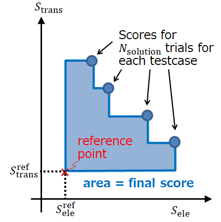* **Final Score**: Based of the equations, $N_{\mathrm{solution}}$ pairs of the scores for transportation and electricity management $\left( =(S_{\mathrm{ele}}^{(1)},S_{\mathrm{trans}}^{(1)}),...,(S_{\mathrm{ele}}^{(N_{\mathrm{solution}})},S_{\mathrm{trans}}^{(N_{\mathrm{solution}})}) \right)$ are plotted on the 2-dimensional plane as in the figure below. For a given reference point, the final score of each test case is determined by the area below. Here, if one of the scores is below those of the reference point, the score is set to the corresponding score of the reference point. By doing that the final score cannot be negative. For the concrete position of the reference point, see "Constraints for Input and Output" * **Standings**: During the contest the total score of a submission is determined by summing the final score of the submission with respect to 16 test cases. Among these test cases, the numbers of sunny without downpour, sunny with downpour, rainy without sudden clear sky, and rainy with sudden clear sky are fixed at 6, 2, 6, and 2, respectively. After the contest a system test will be performed. To this end, the contestant's last submission will be scored by summing the final score of the submission on $200$ previously unseen test cases. Please see the table below for a breakdown of the $200$ test cases. Predicted energy balance (disclosed) Predicted energy balance (undisclosed) Total Sunny without downpour 60 15 75 Sunny with downpour 20 5 25 Rainy without sudden clear sky 60 15 75 Rainy with sudden clear sky 20 5 25 Total 160 40 200 Of the $200$ test cases, $160$ use $6(=N_\mathrm{pattern} \times 2($sunny, rainy$))$ types of predicted energy balance already disclosed in the toolkit. The remaining $40$ test cases use $6(=N_\mathrm{pattern} \times 2($sunny, rainy$))$ types of predicted energy balance that are not disclosed to the contestants. $\Delta_{\mathrm{event}}$, $p_{\mathrm{event}}$, and percentage of nanogrids hit by downpour or sudden clear sky are all the same among $50(=25$\[sunny with downpour\]$+25$\[rainy with sudden clear sky\]$)$ test cases. We are very sorry that the system test specifications have changed unlike the answer to the question received from Mr. yuusanlondon on December 18. As a result of consideration, the organizers of the contest have determined to decide the final standings based on this specification. We appreciate your understanding. (12/29 postscript) Generation method or generator for undisclosed predicted energy balance will not be released. Patterns of undisclosed predicted energy balance are generated so that the full score for Electricity Management using undisclosed predicted energy balance is comparable to that using disclosed predicted energy balance. (Note that the full score means the upper limit of the score by applying an ideal control method.)  Problem B --------- Problem B is an interactive problem similar to problem A. Each contestant is asked to consider the trade-offs between transportation and electricity management and to find $N_{\mathrm{solution}}$ solutions for each test case so that each solution is as close as the trade-off curve and the whole solutions cover a broad range of the trade-off curve. Each contestant and a host machine (judge) interact with the following protocol. Iterative process Contestant Judge Output $N_{\mathrm{solution}}$ Output $G$ Output the weather $\mathrm{DayType}$ Output the information related to energy balance Output the information about the nanogrid Output the information about EV Output the information about the transportation Output the information about the score Output $T_\mathrm{max}$ **for** $i=1,...,N_{\mathrm{solution}}$ **do** **for** $t=0,...,T_\mathrm{max}-1$ **do** \- \- Output $\mathrm{info}_t$ (the status of EVs and nanogrids at the time $t$) Output operations for each EV **end for** Output $\mathrm{info}_t$ (the status of EVs and nanogrids at the time $t=T_\mathrm{max}$) Output score for transportation $S_{\mathrm{trans}}$ and score for electricity management $S_{\mathrm{ele}}$ **end for** The number of trials, the graph $G$, the weather $\mathrm{DayType}$, the information related to energy balance, the nanogrid, EVs and its transportation, the score, $T_\mathrm{max}$ are outputted only once in the beginning of each test case. For each trial, contestants are supposed to interact with judges $T_\mathrm{max}$ times. **Note that $\mathrm{info}_t$ and the scores at the time $t=T_\mathrm{max}$ must be read by the contestant code (otherwise it may be TLE).** Input and Output Format 1 ------------------------- In the beginning of each test case, the number of trials, the graph $G$, the weather $\mathrm{DayType}$, the information related to energy balance, the nanogrid, EVs and its transportation, the score, $T_\mathrm{max}$ is provided through the standard input. Note that the information is provided only once in the beginning of each test case since it is common for all trials. $N_{\mathrm{solution}}$ $|V|$ $|E|$ $u_1$ $v_1$ $d_1$ : $u_{|E|}$ $v_{|E|}$ $d_{|E|}$ $\mathrm{DayType}$ $N_\mathrm{div}$ $N_\mathrm{pattern}$ $\sigma^{2}_{\mathrm{ele}}$ $p_{\mathrm{event}}$ $\Delta_{\mathrm{event}}$ $\mathrm{pw}_{1,1}^{\mathrm{predict}}$ $\mathrm{pw}_{1,2}^{\mathrm{predict}}$ ... $\mathrm{pw}_{1,N_\mathrm{div}}^{\mathrm{predict}}$ : $\mathrm{pw}_{N_\mathrm{pattern},1}^{\mathrm{predict}}$ $\mathrm{pw}_{N_\mathrm{pattern},2}^{\mathrm{predict}}$ ... $\mathrm{pw}_{N_\mathrm{pattern},N_\mathrm{div}}^{\mathrm{predict}}$ $N_\mathrm{grid}$ $C_{\mathrm{init}}^{\mathrm{grid}}$ $C_{\mathrm{max}}^{\mathrm{grid}}$ $V_{\max}^{\mathrm{grid}}$ $x_1$ $\mathrm{pattern}_1$ : $x_{N_\mathrm{grid}}$ $\mathrm{pattern}_{N_\mathrm{grid}}$ $N_\mathrm{EV}$ $C_{\mathrm{init}}^{\mathrm{EV}}$ $C_{\mathrm{max}}^{\mathrm{EV}}$ $V_{\max}^{\mathrm{EV}}$ $N_{\max}^{\mathrm{trans}}$ $\Delta_{\mathrm{move}}^{\mathrm{EV}}$ $\mathrm{pos}_1$ : $\mathrm{pos}_{N_\mathrm{EV}}$ $p_{\mathrm{trans}}^{\mathrm{const}}$ $T_\mathrm{last}$ $P^{\mathrm{trans}}$ $\gamma$ $S_{\mathrm{ele}}^{\mathrm{ref}}$ $S_{\mathrm{trans}}^{\mathrm{ref}}$ $T_\mathrm{max}$ * In the $1$st line, $N_{\mathrm{solution}}$ is the number of trials for each test case. * In the following line, the number of vertices $|V|$ and the number of edges $|E|$ of the graph $G$ are provided. * In the following $|E|$ lines, the edges of the graph along with their weights are provided. The $i$\-th line of the lines indicate that there exists an edge connecting $u_{i}$ and $v_{i}$ with the edge weight $d_i$. * In the following $1$ line, the weather pattern $\mathrm{DayType}$ is provided, which is either $\mathrm{DayType}$ $0$ (sunny without downpour), $1$ (sunny with downpour), $2$ (rainy without sudden clear sky), or $3$ (rainy with sudden clear sky). * In the following $1$ line, the number of subintervals of equal length on which the predicted energy balance is constant $N_\mathrm{div}$, the number of possible patterns of the time series of predicted energy balance $N_\mathrm{pattern}$, the variance of the stochastic fluctuation of the difference $\sigma^{2}_{\mathrm{ele}}$, the probability of occurrences of downpour or sudden clear $p_{\mathrm{event}}$ ($p_{\mathrm{event}}=0.0$ in the case of $\mathrm{DayType}=0$ or $2$), and the variation of energy balance in case of downpour or sudden clear sky $\Delta_{\mathrm{event}}$. * In the following $N_\mathrm{pattern}$ lines, the time series of predicted energy balance is provided. The $j$\-th element in the $i$\-th line of the lines ($\mathrm{pw}_{i,j}^{\mathrm{predict}}$) indicates the predicted energy balance of the $j$\-th subinterval in case of the $i$\-th pattern. * In the following $1$ line, the number of nanogrids $N_\mathrm{grid}$ and the initial value of the charged capacity of the battery for each nanogrid $C_{\mathrm{init}}^{\mathrm{grid}}$ ($t=0$), the upper limit of the charged capacity of the battery $C_{\mathrm{max}}^{\mathrm{grid}}$, and the maximum charge/discharge speed of the battery $V_{\max}^{\mathrm{grid}}$ is provided. * In the following $N_\mathrm{grid}$ lines, the information about each nanogrid is provided. In the $N_\mathrm{grid}$ lines, the $i$\-th line indicates that a nanogrid is located on the vertex $x_i$ whose pattern of the time series of predicted energy balance is $\mathrm{pattern}_i$. * In the following $1$ line, the number of EVs $N_\mathrm{EV}$, their initial charged capacity $C_{\mathrm{init}}^{\mathrm{EV}}$, their maximum charged capacity $C_{\mathrm{max}}^{\mathrm{EV}}$, and their maximum charge/discharge speed $V_{\max}^{\mathrm{EV}}$, the maximum number orders each EV can carry on $N_{\max}^{\mathrm{trans}}$, and the amount of electricity necessary for each EV to travel in a unit distance $\Delta_{\mathrm{move}}^{\mathrm{EV}}$. * In the following $N_\mathrm{EV}$ lines, the position of each EV is provided. In the $N_\mathrm{EV}$ line, the $i$\-th line indicates that the $i$\-th EV is located on the vertex $\mathrm{pos}_i$. * In the following $1$ line, the probability that a new order is generated $p_{\mathrm{trans}}^{\mathrm{const}}$ and the last time when a new order can be generated $T_\mathrm{last}$. * In the following $1$ line, the penalty for the outstanding order $P^{\mathrm{trans}}$, the proportional constant $\gamma$ for the penalty of getting power supply from outside, the reference score of electricity management $S_{\mathrm{ele}}^{\mathrm{ref}}$, and for transportation $S_{\mathrm{trans}}^{\mathrm{ref}}$ are provided. * In the last line, the total time step for each trial of each test case $T_{\max}$ is provided. Input and Output Format 2 ------------------------- For each time $t$, contestants get the status of EVs and nanogrids $\mathrm{info}_t$ from the standard input. $x_1$ $y_1$ $\mathrm{pw}_{1}^{\mathrm{actual},t-1}$ $\mathrm{pw}_{1}^{\mathrm{excess},t-1}$ $\mathrm{pw}_{1}^{\mathrm{buy},t-1}$ : $x_{N_\mathrm{grid}}$ $y_{N_\mathrm{grid}}$ $\mathrm{pw}_{N_\mathrm{grid}}^{\mathrm{actual},t-1}$ $\mathrm{pw}_{N_\mathrm{grid}}^{\mathrm{excess},t-1}$ $\mathrm{pw}_{N_\mathrm{grid}}^{\mathrm{buy},t-1}$ $\mathrm{carinfo}_1$ : $\mathrm{carinfo}_{N_\mathrm{EV}}$ $N_\mathrm{order}$ $\mathrm{id}_1$ $w_1$ $z_1$ $\mathrm{state}_1$ $\mathrm{time}_1$ ... $\mathrm{id}_{N_\mathrm{order}}$ $w_{N_\mathrm{order}}$ $z_{N_\mathrm{order}}$ $\mathrm{state}_{N_\mathrm{order}}$ $\mathrm{time}_{N_\mathrm{order}}$ * In the $N_\mathrm{grid}$ lines, the $i$\-th line indicates the charged capacity of the battery of the nanogrid on the vertex $x_i$ is $y_i$, and $\mathrm{pw}_{i}^{\mathrm{actual},t-1}$, $\mathrm{pw}_{i}^{\mathrm{excess},t-1}$, and $\mathrm{pw}_{i}^{\mathrm{buy},t-1}$ indicate actual energy balance, excess amount of power discarded, and power supplied from the outside at the previous time step $t-1$, respectively. At $t=0$, $\mathrm{pw}_{i}^{\mathrm{actual},t-1}$, $\mathrm{pw}_{i}^{\mathrm{excess},t-1}$, and $\mathrm{pw}_{i}^{\mathrm{buy},t-1}$ are all displayed as $0$. Note that $\mathrm{pw}_{i}^{\mathrm{actual},t-1}$, $\mathrm{pw}_{i}^{\mathrm{excess},t-1}$, and $\mathrm{pw}_{i}^{\mathrm{buy},t-1}$ correspond to $\Delta^{\mathrm{grid}}_{\mathrm{gen},t-1}$, $\Delta^{\mathrm{grid}}_{\mathrm{total},t-1} - \min \left{ V_{\max}^{\mathrm{grid}}, C^{\mathrm{grid}}_{\max}-C^{\mathrm{grid}}_{t-1} \right}$, and $- \Delta^{\mathrm{grid}}_{\mathrm{total},t-1} - \min \left{ V_{\max}^{\mathrm{grid}}, C^{\mathrm{grid}}_{t-1} \right}$, respectively (see [Charge/Discharge to the Battery of a Nanogrid](#charge_en) ). If "step 2" and "step 3" are not executed at the previous time $t−1$, $\mathrm{pw}_{i}^{\mathrm{excess},t-1}$ and $\mathrm{pw}_{i}^{\mathrm{buy},t-1}$ are 0, respectively. * In the following $N_\mathrm{EV}$ groups of $4$ lines, the $i$\-th group $\mathrm{carinfo}_i$ indicated the status of the $i$\-th EV. For the detail, see the information below. * In the following $1$ line, the number of outstanding orders up to the time $t$ $N_\mathrm{order}$ is provided. * In the following $N_\mathrm{order}$ lines, the $i$\-th line indicates that the starting and destination points of order with ID $\mathrm{id_i}$ are $w_i$ and $z_i$, respectively, and the state of the order is $\mathrm{state}_i$ and the order is generated at the time $\mathrm{time}_1$, where $\mathrm{state}_i=0$ indicates none of the EVs picked it up and $\mathrm{state}_i=1$ indicates one of the EVs picked it up but it is not yet delivered. Here, $\mathrm{carinfo}_i$ is provided in the following format. $\mathrm{charge}_i$ $u_i$ $v_i$ $\mathrm{dist_from}_u_i$ $\mathrm{dist_to}_v_i$ $N_{\mathrm{adj},i}$ $a_{i,1}$ $a_{i,2}$ $\ldots$ $a_{i,N_\mathrm{adj}}$ $N_{\mathrm{order},i}$ $o_{i,1}$ $o_{i,2}$ $\ldots$ $o_{N_{\mathrm{order}, i}}$ * The first line indicates that the charged capacity of the $i$\-th EV is $\mathrm{charge}_i$. * The second line indicates the present position of $i$\-th. If $u_i \ne v_i$ holds, the $i$\-th EV is on the edge connecting $u_i$ and $v_i$, and the distance to the vertex $u_i$ is $\mathrm{dist_from}_u_i$ and that to $v_i$ is $\mathrm{dist_to}_v_i$. If $u_i = v_i$ holds, the $i$\-th EV is on the vertex $u_i$ (in this case, both $\mathrm{dist_from}_u_i$ and $\mathrm{dist_to}_v_i$ are displayed as $0$). * The third line indicates that there are $N_{\mathrm{adj},i}$ possible vertices to which the $i$ EV moves by the operation `move` and $a_{i,1}$, $a_{i,2}$、$\ldots$ and $a_{i,N_\mathrm{adj}}$ are the possible vertices. * The fourth line indicates there are $N_{\mathrm{order},i}$ orders put on the $i$\-th EV and the IDs of the orders are $o_{i,1}$, $o_{i,2}$, $\ldots$, $o_{N_{\mathrm{order}, i}}$. In responding to the input, contestants are asked to output the operation of each EV $\mathrm{command}_i$ $(1 \leq i \leq N_\mathrm{EV})$ for each time $t$ ($0 \leq t \lt T_{\max}$). Each operation should be separated by the new line and the output should end with the new line. $\mathrm{command}_{1}$ $\mathrm{command}_{2}$ : $\mathrm{command}_{N_\mathrm{EV}}$ Here, $\mathrm{command}$ should be in the following format. There are five possible operations `stay`, `move w`, `pickup a`, `charge_from_grid`, and `charge_to_grid` for each EV. Contestants should choose one of them for each EV and output it in one line as follows: * `stay` * `move w` * `pickup a` * `charge_from_grid` $\Delta^{\mathrm{grid} \rightarrow \mathrm{EV}}_{\mathrm{charge}}$ * `charge_to_grid` $\Delta^{\mathrm{EV} \rightarrow \mathrm{grid}}_{\mathrm{charge}}$ There are constraints for each operation (See [EV](#ev_en) **Operation for EVs** for the detail). The behavior of the judge when one of these constraints is violated is undefined. Input and Output Format 3 ------------------------- After the operation of each EV at $t=T_\mathrm{max}-1$ is output, $\mathrm{info}_t$ at $t=T_\mathrm{max}$ is provided through the standard input from the judge (the format of $\mathrm{info}_t$ is the same as the format written in Input/Output format 2). On the next line, then, the judge gives the score for transportation $S_{\mathrm{trans}}$ and the score for electricity management $S_{\mathrm{ele}}$ to the standard input in the following format. $S_{\mathrm{trans}}$ $S_{\mathrm{ele}}$ Constraints for Input and Output -------------------------------- * Of the following numbers, those described as **"\[float\]"** are given as floats, and the others are given as integers. #### Input and output format 1 provided in the beginning of each test case * $N_{\mathrm{solution}} = 5$ * $|V| = 225$ * $1.5 |V| \leq |E| \leq 2 |V|$ * $1 \leq u_{i}, v_{i} \leq |V|, u_i \ne v_i$ $(1 \leq i \leq |E|)$ * $1 \leq d_i \leq \lceil 2\sqrt{2|V|} \rceil$ $(1 \leq i \leq |E|)$ * The graph $G$ is guaranteed to be simple and connected. * $\mathrm{DayType} \in \left{ 0, 1, 2, 3 \right}$ * $N_\mathrm{div} = 20$ * $N_\mathrm{pattern} = 3$ * $\sigma^{2}_{\mathrm{ele}} = 100$ * $p_{\mathrm{event}} \in \left{ 0.0, 0.1 \right}$ **"\[float\]"** * $\Delta_{\mathrm{event}} = 1000$ * $-1000 \lt \mathrm{pw}_{i,j}^{\mathrm{predict}} \lt 1000 (1 \leq i \leq N_\mathrm{pattern}, 1 \leq j \leq N_\mathrm{div})$ * $N_\mathrm{grid} = 20$ * $C_{\mathrm{init}}^{\mathrm{grid}} = 25000$ * $C_{\mathrm{max}}^{\mathrm{grid}} = 50000$ * $V_{\max}^{\mathrm{grid}} = 800$ * $1 \leq x_i \leq |V|$ (if $i \neq j$, $x_i \neq x_j. 1 \leq i \leq N_\mathrm{grid})$ * $1 \leq \mathrm{pattern}_i \leq N_\mathrm{pattern}$ $(1 \leq i \leq N_\mathrm{grid})$ * $N_{\min}^{\mathrm{EV}} = 15$ * $N_{\max}^{\mathrm{EV}} = 25$ * $N_{\min}^{\mathrm{EV}} \leq N_\mathrm{EV} \leq N_{\max}^{\mathrm{EV}}$ * $C_{\mathrm{init}}^{\mathrm{EV}} = 12500$ * $C_{\mathrm{max}}^{\mathrm{EV}} = 25000$ * $V_{\max}^{\mathrm{EV}} = 400$ * $N_{\max}^{\mathrm{trans}} = 4$ * $\Delta_{\mathrm{move}}^{\mathrm{EV}} = 50$ * $1 \leq \mathrm{pos}_i \leq |V| (1 \leq i \leq N_\mathrm{EV})$ * $p_{\mathrm{trans}}^{\mathrm{const}} = 0.7$ **"\[float\]"** * $T_\mathrm{last} = 900$ * $P^{\mathrm{trans}} = 3000$ * $\gamma = 2.0$ **"\[float\]"** * $S_{\mathrm{ele}}^{\mathrm{ref}} = -1,500,000$ * $S_{\mathrm{trans}}^{\mathrm{ref}} = -1,900,000$ * $T_\mathrm{max} = 1000$ #### Input and output format 2 provided for each time step * $1 \leq x_i \leq |V|$ (if $i \neq j$, $x_i \neq x_j. 1 \leq i \leq N_\mathrm{grid})$ * $0 \leq y_i \leq C_{\mathrm{max}}^{\mathrm{grid}}$ $(1 \leq i \leq N_\mathrm{grid})$ * $-10000 \lt \mathrm{pw}_{i}^{\mathrm{actual},j} \lt 10000 (1 \leq i \leq N_\mathrm{grid}, -1 \leq j \leq T_\mathrm{max}-2)$ * $0 \leq \mathrm{pw}_{i}^{\mathrm{excess},j} \lt 10000, (1 \leq i \leq N_\mathrm{grid}, -1 \leq j \leq T_\mathrm{max}-2)$ * $0 \leq \mathrm{pw}_{i}^{\mathrm{buy},j} \lt 10000, (1 \leq i \leq N_\mathrm{grid}, -1 \leq j \leq T_\mathrm{max}-2)$ * $0 \leq \mathrm{charge}_i \leq C_{\mathrm{max}}^{\mathrm{EV}}$ $(1 \leq i \leq N_\mathrm{EV})$ * $1 \leq u_i, v_i \leq |V|$ $(1 \leq i \leq N_\mathrm{EV})$ * $0 \leq \mathrm{dist_from}_u_i \leq \lceil 2\sqrt{2|V|} \rceil$ $(1 \leq i \leq N_\mathrm{EV})$ * $0 \leq \mathrm{dist_to}_v_i \leq \lceil 2\sqrt{2|V|} \rceil$ $(1 \leq i \leq N_\mathrm{EV})$ * $1 \leq N_{\mathrm{adj},i} \leq 5(\mathrm{MaxDegree})$ $(1 \leq i \leq N_\mathrm{EV})$ * $1 \leq a_{i,j} \leq |V|$ $(1 \leq i \leq N_\mathrm{EV}, 1 \leq j \leq N_{\mathrm{adj},i})$ * $0 \leq N_{\mathrm{order},i} \leq N_{\max}^{\mathrm{trans}}$ $(1 \leq i \leq N_\mathrm{EV})$ * $1 \leq o_{i,j} \leq T_\mathrm{last}$ $(1 \leq i \leq N_\mathrm{EV}, 1 \leq j \leq N_{\mathrm{order},i})$ * $0 \leq N_\mathrm{order} \leq T_\mathrm{last}$ * $1 \leq \mathrm{id}_i \leq T_\mathrm{last}$ $(1 \leq i \leq N_\mathrm{order})$ * $1 \leq w_i \leq |V|$ $(1 \leq i \leq N_\mathrm{order})$ * $1 \leq z_i \leq |V|$ $(1 \leq i \leq N_\mathrm{order})$ * $w_i \ne z_i$ $(1 \leq i \leq N_\mathrm{order})$ * $\mathrm{state}_i \in \left{ 0, 1 \right}$ $(1 \leq i \leq N_\mathrm{order})$ * $0 \leq \mathrm{time}_i \leq T_\mathrm{last}$ $(1 \leq i \leq N_\mathrm{order})$ #### Input and output format 3 provided at the end of each test case * $S_{\mathrm{trans}}$ **"\[float\]"** * $S_{\mathrm{ele}}$ **"\[float\]"** Example of Inputs and Outputs ----------------------------- * * * Note: This example is to explain how a judge and a contestant interact with each other through inputs and outputs. To simplify the explanation, some of the parameter values like the number of vertices are set to small and they may be outside of the ranges in Constraints of Input and Output. For example, the number of vertices is set to $4$ in this example but is set to $225$ in each test case. .pre-sample-inout { margin: 0; } Time Step Judge Contestant Explanation 1 4 4 1 2 1 2 3 2 3 4 3 4 1 1 0 2 2 1 0 10 5 -2 -4 4 2 10 20 4 1 1 4 2 2 5 10 2 2 1 2 4 0.5 3 3 0.5 -100 -100 4 Initial parameter values are provided by Judge in the beginning of each test case Line $1$: $N_{\mathrm{solution}}$ is $1$. Line $2$: Graph $G$ consists of $|V| = 4$ vertices and $|E| = 4$ edges. The following $4$ lines (Line $3$ - Line $6$) indicate the edges of the graph. Line $3$: Edge $1$ connects the vertex $1$ and $2$ and its distance is $1$. Line $4$: Edge $2$ connects the vertex $2$ and $3$ and its distance is $2$. Line $5$: Edge $3$ connects the vertex $3$ and $4$ and its distance is $3$. Line $6$: Edge $4$ connects the vertex $4$ and $1$ and its distance is $1$. Line $7$: The weather pattern in this test case is $0$ "Sunny without downpour". Line $8$: $N_{\mathrm{div}}$ is $2$, $N_\mathrm{pattern}$ is $2$, $\sigma^{2}_{\mathrm{ele}}$ is $1$, $p_{\mathrm{event}}$ is $0$, $\Delta_{\mathrm{event}}$ is $10$. The following $2$ lines (Line $9$ - Line $10$) indicate the predicted energy balance. Line $9$: The predicted energy balance of nanogrids having the demand pattern $1$ is $5$ for the $1$\-st time interval and $-2$ for the $2$\-nd time interval. Line $10$: The predicted energy balance of nanogrids having the demand pattern $1$ is $-4$ for the $1$\-st time interval and $4$ for the $2$\-nd time interval. Line $11$: $N_\mathrm{grid} = 2$, $C_{\mathrm{init}}^{\mathrm{grid}} = 10$, $C_{\mathrm{max}}^{\mathrm{grid}} = 20$ and $V_{\max}^{\mathrm{grid}} = 4$. Line $12$: Nanogrid $1$ is on the vertex $1$ and it has the demand pattern $1$. Line $13$: Nanogrid $2$ is on the vertex $4$ and it has the demand pattern $2$. Line $14$: $N_\mathrm{EV} = 2$, $C_{\mathrm{init}}^{\mathrm{EV}} = 5$, $C_{\mathrm{max}}^{\mathrm{EV}} = 10$, $V_{\max}^{\mathrm{EV}} = 2$, $N_{\max}^{\mathrm{trans}} = 2$, and $\Delta_{\mathrm{move}}^{\mathrm{EV}} = 1$. The following $2$ lines (Line $15$ - Line $16$) indicate the positions of the EVs at time $t=0$. Line $15$: EV $1$ is on the vertex $2$ at time $t=0$. Line $16$: EV $2$ is on the vertex $4$ at time $t=0$. Line $17$: $p_{\mathrm{trans}}^{\mathrm{const}} = 0.5$ and $T_\mathrm{last} = 3$. Line $18$: $P^{\mathrm{trans}} = 3$, $\gamma = 0.5$, $S_{\mathrm{ele}}^{\mathrm{ref}} = -100$ and $S_{\mathrm{trans}}^{\mathrm{ref}} = -100$. Line $19$: $T_{\max} = 4$. 0 1 10 0 0 0 4 10 0 0 0 5 2 2 0 0 2 1 3 0 5 4 4 0 0 2 1 3 0 1 1 1 4 0 0 move 1 charge_from_grid 2 Input data at time $0$ is provided by Judge. Line 1: The charged capacity of the nanogrid at the vertex $1$ at time $0$ is $10$. All the other three values are irrelevant at time $0$ and are set to $0$. Line 2: The charged capacity of the nanogrid at the vertex $4$ at time $0$ is $10$. All the other three values are irrelevant at time $0$ and are set to $0$. The following $4$ lines (Line $3$ - Line $6$) indicate the status of EV $1$. Line 3: The charged capacity of EV $1$ is $5$ at time $0$. Line 4: EV $1$ is on the vertex $2$ at time $0$. Line 5: There are $N_{\mathrm{adj},1} = 2$ vertices toward which EV $1$ can \`move\` and the vertices are $1$ and $3$. Line 6: The number of orders on EV $1$ is $N_{\mathrm{order},i} = 0$. The following $4$ lines (Line $7$ - Line $10$) indicate the status of EV $2$. Line 7: The charged capacity of EV $2$ is $5$ at time $0$. Line 8: EV $2$ is on the vertex $4$ at time $0$. Line 9: There are $N_{\mathrm{adj},1} = 2$ vertices toward which EV $2$ can \`move\` and the vertices are $1$ and $3$. Line 10: The number of orders on EV $2$ is $N_{\mathrm{order},i} = 0$. Line 11: There is $N_\mathrm{order} = 1$ outstanding order. Line 12: The starting and destination vertices of the order $1$ are $1$ and $4$ respectively. The order is not on any EVs and is generated at time $0$. Output from Contestant Line 1: Operate EV $1$ to move toward the vertex $1$. If the charged capacity of EV $1$ is less than $1$, EV $1$ cannot move as operated. In this case, the charged capacity of EV $1$ is $5$ and thus EV $1$ moves toward the vertex $1$ by the distance $1$ by consuming electricity by $1$ in the next time step. Since the road distance of the edge connecting the vertices $1$ and $2$ is $1$, the location of EV $1$ is the vertex $1$ in the next time step. Line 2: EV $2$ charges from the nanogrid by $2$. This operation does not violate the constraints because EV $2$ is on the vertex $4$ where the nanogrid is located, the charged amount $2$ does not exceeds the maximum charge speeds of EV and the battery of the nanogrid. Since the resulting charged capacity of EV $2$ is $7$, which is less than the maximum charged capacity of EV ($10$), the resulting charged capacity of EV $2$ is $7$ in the next time step. 1 1 14 5 1 0 4 6 -4 0 2 4 1 1 0 0 2 2 4 0 7 4 4 0 0 2 1 3 0 1 1 1 4 0 0 pickup 1 charge_from_grid 2 Input data at time $1$ is provided by Judge. Line 1: The charged capacity of the nanogrid on the vertex $1$ at time $1$ is $14$. The actual energy balance, the amount of electricity overflowed, and the amount of the electricity supplied from the outside at time $0$ are $5, 1, 0$ , respectively. Line 2: The charged capacity of the nanogrid on the vertex $4$ at time $1$ is $6$. The actual energy balance, the amount of electricity overflowed, and the amount of the electricity supplied from the outside at time $0$ are $-4, 0, 2$ , respectively. The following $4$ lines (Line $3$ - Line $6$) indicate the status of EV $1$. Line 3: The charged capacity of EV $1$ is $4$ at time $1$. Line 4: EV $1$ is on the vertex $1$ at time $1$. Line 5: There are $N_{\mathrm{adj},1} = 2$ vertices toward which EV $1$ can \`move\` and the vertices are $2$ and $4$. Line 6: The number of orders on EV $1$ is $N_{\mathrm{order},i} = 0$. The following $4$ lines (Line $7$ - Line $10$) indicate the status of EV $2$. Line 7: The charged capacity of EV $2$ is $7$ at time $1$. Line 8: EV $2$ is on the vertex $4$ at time $1$. Line 9: There are $N_{\mathrm{adj},1} = 2$ vertices toward which EV $2$ can \`move\` and the vertices are $1$ and $3$. Line 10: The number of orders on EV $2$ is $N_{\mathrm{order},i} = 0$. Line 11: There is $N_\mathrm{order} = 1$ outstanding order. Line 12: The starting and destination vertices of the order $1$ are $1$ and $4$ respectively. The order is not on any EVs and is generated at time $1$. Output from Contestant Line 1: Locate the order $1$ on EV $1$. EV $1$ does not consume electricity by this operation. Line 2: EV $2$ charges from the nanogrid by $2$. This operation does not violate the constraints because EV $2$ is on the vertex $4$ where the nanogrid is located, the charged amount $2$ does not exceeds the maximum charge speeds of EV and the battery of the nanogrid. Since the resulting charged capacity of EV $2$ is $9$, which is less than the maximum charged capacity of EV ($10$), the resulting charged capacity of EV $2$ is $9$ in the next time step. 2 1 18 5 1 0 4 2 -4 0 2 4 1 1 0 0 2 2 4 1 1 9 4 4 0 0 2 1 3 0 2 1 1 4 1 0 2 4 1 0 2 move 4 pickup 2 Input data at time $2$ is provided by Judge. Line 1: The charged capacity of the nanogrid on the vertex $1$ at time $2$ is $18$. The actual energy balance, the amount of electricity overflowed, and the amount of the electricity supplied from the outside at time $1$ are $5, 1, 0$ , respectively. Line 2: The charged capacity of the nanogrid on the vertex $4$ at time $2$ is $2$. The actual energy balance, the amount of electricity overflowed, and the amount of the electricity supplied from the outside at time $1$ are $-4, 0, 2$ , respectively. The following $4$ lines (Line $3$ - Line $6$) indicate the status of EV $1$. Line 3: The charged capacity of EV $1$ is $4$ at time $2$. Line 4: EV $1$ is on the vertex $1$ at time $2$. Line 5: There are $N_{\mathrm{adj},1} = 2$ vertices toward which EV $1$ can \`move\` and the vertices are $2$ and $4$. Line 6: The number of orders on EV $1$ is $N_{\mathrm{order},i} = 1$ and that the ID of the order is $1$. The following $4$ lines (Line $7$ - Line $10$) indicate the status of EV $2$. Line 7: The charged capacity of EV $2$ is $9$ at time $2$. Line 8: EV $2$ is on the vertex $4$ at time $2$. Line 9: There are $N_{\mathrm{adj},1} = 2$ vertices toward which EV $2$ can \`move\` and the vertices are $1$ and $3$. Line 10: The number of orders on EV $2$ is $N_{\mathrm{order},i} = 0$. Line 11: There are $N_\mathrm{order} = 2$ outstanding orders. Line 12: The starting and destination vertices of the order $1$ are $1$ and $4$ respectively. The order is on an EV and is generated at time $0$. Line 13: The starting and destination vertices of the order $2$ are $4$ and $1$ respectively. The order is not on any EV and is generated at time $2$. Output from Contestant Line 1: Operate EV $1$ to move toward the vertex $4$. If the charged capacity of EV $1$ is less than $1$, EV $1$ cannot move as operated. In this case, the charged capacity of EV $1$ is $4$ and thus EV $1$ moves toward the vertex $4$ by the distance $1$ by consuming electricity by $1$ in the next time step. Since the road distance of the edge connecting the vertices $1$ and $4$ is $1$, the location of EV $1$ is the vertex $4$ in the next time step. Line 2: Locate the order $2$ on EV $2$. EV $2$ does not consume electricity by this operation. 3 1 17 -1 0 0 4 6 4 0 0 3 4 4 0 0 2 1 3 0 9 4 4 0 0 2 1 3 1 2 1 2 4 1 1 2 stay move 1 Input data at time $3$ is provided by Judge. Line 1: The charged capacity of the nanogrid on the vertex $1$ at time $3$ is $17$. The actual energy balance, the amount of electricity overflowed, and the amount of the electricity supplied from the outside at time $2$ are $-1, 0, 0$ , respectively. Line 2: The charged capacity of the nanogrid on the vertex $4$ at time $3$ is $6$. The actual energy balance, the amount of electricity overflowed, and the amount of the electricity supplied from the outside at time $2$ are $4, 0, 0$ , respectively. The following $4$ lines (Line $3$ - Line $6$) indicate the status of EV $1$. Line 3: The charged capacity of EV $1$ is $3$ at time $3$. Line 4: EV $1$ is on the vertex $4$ at time $3$. Line 5: There are $N_{\mathrm{adj},1} = 2$ vertices toward which EV $1$ can \`move\` and the vertices are $1$ and $3$. Line 6: The number of orders on EV $1$ is $N_{\mathrm{order},i} = 0$. Since the destination vertex of the order $1$ is $4$ and EV $1$ is arrived at the vertex, the order $1$ is delivered. The following $4$ lines (Line $7$ - Line $10$) indicate the status of EV $2$. Line 7: The charged capacity of EV $2$ is $9$ at time $3$. Line 8: EV $2$ is on the vertex $4$ at time $3$. Line 9: There are $N_{\mathrm{adj},1} = 2$ vertices toward which EV $2$ can \`move\` and the vertices are $1$ and $3$. Line 10: The number of orders on EV $2$ is $N_{\mathrm{order},i} = 1$ and the ID of the order is $2$. Line 11: There are $N_\mathrm{order} = 1$ outstanding orders. Line 12: The starting and destination vertices of the order $2$ are $4$ and $1$ respectively. The order is on an EV and is generated at time $2$. Output from Contestant Line 1: EV $1$ stays on the same vertex. Line 2: Operate EV $2$ to move toward the vertex $1$. If the charged capacity of EV $2$ is less than $1$, EV $2$ cannot move as operated. In this case, the charged capacity of EV $2$ is $9$ and thus EV $2$ moves toward the vertex $1$ by the distance $1$ by consuming electricity by $1$ in the next time step. Since the road distance of the edge connecting the vertices $4$ and $1$ is $1$, the location of EV $2$ is the vertex $1$ in the next time step. 4 1 15 -2 0 0 4 10 5 1 0 3 4 4 0 0 2 1 3 0 8 1 1 0 0 2 2 4 0 0 3.0 34.0 Input data at time $4$ is provided by Judge. Line 1: The charged capacity of the nanogrid on the vertex $1$ at time $4$ is $15$. The actual energy balance, the amount of electricity overflowed, and the amount of the electricity supplied from the outside at time $3$ are $-2, 0, 0$ , respectively. Line 2: The charged capacity of the nanogrid on the vertex $4$ at time $4$ is $6$. The actual energy balance, the amount of electricity overflowed, and the amount of the electricity supplied from the outside at time $3$ are $5, 1, 0$ , respectively. The following $4$ lines (Line $3$ - Line $6$) indicate the status of EV $1$. Line 3: The charged capacity of EV $1$ is $3$ at time $4$. Line 4: EV $1$ is on the vertex $4$ at time $4$. Line 5: There are $N_{\mathrm{adj},1} = 2$ vertices toward which EV $1$ can \`move\` and the vertices are $1$ and $3$. Line 6: The number of orders on EV $1$ is $N_{\mathrm{order},i} = 0$. The following $4$ lines (Line $7$ - Line $10$) indicate the status of EV $2$. Line 7: The charged capacity of EV $2$ is $8$ at time $4$. Line 8: EV $2$ is on the vertex $4$ at time $4$. Line 9: There are $N_{\mathrm{adj},1} = 2$ vertices toward which EV $2$ can \`move\` and the vertices are $2$ and $4$. Line 10: The number of orders on EV $2$ is $N_{\mathrm{order},i} = 0$. Since the destination vertex of the order $2$ is $1$ and EV $2$ is arrived at the vertex, the order $2$ is delivered. Line 11: There are $N_\mathrm{order} = 0$ outstanding orders. The following $1$ line (Line $12$) indicates the score for transportation and for electricity management. Line 12: The score for transportation is $3.0$ and that for electricity management is $34.0$. How it is scored: The two orders are generated; they are delivered and their waiting times are $3$ and $2$ respectively. Therefore, the score for transportation is calculated by $(4-3)+(4-2)-0=3.0$. In the last time step, the charged capacities of the two EVs are $3$ and $8$ respectively and the charged capacities of the nanogrids are $15$ and $10$ respectively. Therefore, total amount of charged capacity is $36$. In addition, the total amount of electricity supplied from the outside is $4$ (Electricity of the amount $2$ is supplied to the nanogrid on the vertex $4$ from the outside at time $0$ and $1$.) and the amount multiplied by $\gamma$ is subtracted from the score for electricity management. Therefore, the score for electricity is calculated as $36-0.5 \times 4=34.0$. Sample Code B ------------- A software toolkit for generation of input samples (test cases), scoring and testing on a local contestant environment is provided through the following [link](https://img.atcoder.jp/hokudai-hitachi2020/5ab74962545bbb200f633f2a6f1d9fb3.zip). Sample code for beginners is also available. **The toolkit has been updated because minor bugs were found. (December 18th)** **The toolkit that can also be used on windows (Cygwin and WSL) has been released. The English version of the README (short ver.) has also been added. A bug related to constraints has also been fixed. (December 18th)** **The English version of the README (full version) has been released. Also, a small error in the Japanese version of the README has been fixed. (December 21st)** **The toolkit has been updated according to a fix in the judge system regarding submission of the source code written in Python etc. Also, sample code written in Python has been included. Please see the README for how to use it.(January 6th)** **The toolkit has been updated.(A fix regarding DEBUG_LEVEL, etc.) Sample code has also been updated. (January 12th)** * Input sample (test case) generator * Tester * Sample code for beginners [samples]